patrickcleeve2.github.io

Object Tracking

Self driving cars need to understand the world around them, in order to navigate. An important part of this is detecting other objects, such as pedestrians and vehicles, and predicting what they are going to do next. In order to predict what they will do next, we first need to be able to track them over time to understand their movement and behaviour.

Problem

Tracking can be used to solve a number of different problems:

Detections can fail to detect objects for a number of reasons (e.g. model failure, object occlusion). By tracking objects over time we can cover for failures in any given frame by using the previous known position of the object.

Through tracking, we can identify the same object through time which allows us to follow an individual agent. We can then identify properties about it, for example, we might track an individual player on the field to identify their path and actions, or allow a camera drone to follow a person. This problem is sometimes called Re-identification.

Most importantly for self-driving, tracking objects forms a basis for making predictions about what they might do next. From tracking we can determine the velocity of an object, as well as their past behaviour so we can make an informed prediction about where they are going, and what they are trying to do. This is important because we don’t just want to react to objects in the world as that becomes a test of reaction times, and actuation response. Instead we want to predict what will happen next, so we can plan accordingly.For example, we want to predict if a pedestrian is going to cross the road, or if a car is going to merge into our lane.

For this post, we are going to use a couple of small example scenes of pedestrians crossing the road. The scene was collected using the CARLA simulator.


Sequence 1


Sequence 2

To motivate the need for tracking, lets see the output of the object detector.


Sequence 1 Detections

In the first clip, as the pedestrian goes behind the pole, the detector loses them.


Sequence 2 Detections

In the second clip, as the pedestrians get close together the detections become confused by the overlapping, and we again lose a detection.

Definition

There are multiple types of tracking problems, each requiring a different solution.

Single vs Multi Object For single object tracking we are only interested in tracking a single instance of the object through time. This can be a simple case of tracking a single face in a video stream, or a more complicated case of tracking an individual person through a crowd. Multi-object tracking refers to tracking all instances of the object, such as tracking all the people walking through a shopping centre.

Single vs Multi Class Single class tracking assumes that all objects tracked belong to the same class, and doesn’t distinguish between different types of objects. For example, we might only be interested in tracking pedestrians, and filter out any other types of objects we detect. Multi class tracking requires multiple types of objects to be tracked simultaneously. We have to retain a class label for each object we are tracking (such as pedestrian or vehicle).

Online vs Offline Online tracking runs in real time, and objects must be detected, and tracked before the next camera frame can be processed. In this kind of tracking, we only have access to the current frame and any past information about the objects we retain. This is the type of tracking most autonomous systems use in order to move about the world. Offline tracking doesn’t need to be processed in real time, and can use information from the future to improve the tracking algorithm. For example, if the detector loses an object, but picks it back up later, we can use this future information to correct the missing detections and improve our tracking. In addition, these kinds of algorithms can be much more computationally expensive than online tracking. Offline tracking methods are suited to running analysis on a video stream.

Specifically for self-driving, we are interested in multi-object, multi-class, online tracking.

In this post, we are going to be talking about tracking by detection. Using this method, we use a detector to detect objects, and then run a tracker on the detection output. There are other methods for tracking (e.g. optical flow) for different applications.


Optical Flow Example

Methods

Our goal in tracking is to identify the same object in each frame over time. We can come up with some intuitive ways to think about how we might find the same object in different frames.
If there isn’t a lot of time between frames, our object will be in relatively the same position between them. Therefore, if detections in consecutive frames are close to another, then they are likely to belong to the same object. We will call this the Distance metric.

The appearance of our object shouldnt change significantly over time. Therefore, we can compare how our detections look in one frame to another. We will call this the Appearance metric.

Once we have detected an object in a few frames, we can make a rough prediction about how it is moving. Once we have this motion model, we can predict where it is likely to be located in the next frame. We will call this the Motion metric.

Calculating Metrics

Distance

There are a number of different ways to calculate whether two objects are “close” to one another. Some of the most common include:

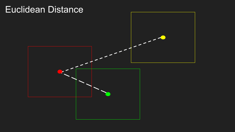
Euclidean distance

The euclidean distance (straight line distance), between the centre of each detection provides a simple way for measuring distance. The distance is measured from the centre point of each bounding box. Euclidean distance is a useful metric as it is fast to calculate, and scales easily to 3-dimensional objects.


Euclidean Distance

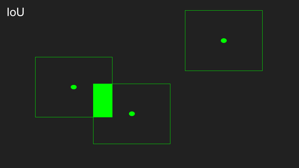
Intersection over Union (IoU)

The IoU method evaluates how much the bounding boxes overlap compared to their overall size. The greater proportion of the bouncing box that overlaps, the higher the IoU score. For bounding boxes that don’t overlap, the IoU is zero, regardless of how close or far away they are.


Intersection over Union

Appearance

Bounding Box Size

The simplest way to compare object appearances is to evaluate the size of the bounding box. As long as the object is not moving very fast, or the perspective isn’t changing significantly, the size of the bounding boxes should be fairly consistent over short time periods, and only change slowly.

Image Similarity

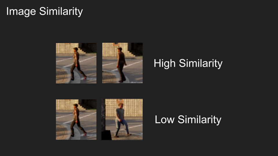
For two different detections we can calculate how ‘similar’ the images inside the bounding boxes are. The assumption is that the same object will appear similar in subsequent frames, when compared to other detected objects. There are a number of methods for calculated similarity, ranging from colour, feature or template matching, to more sophisticated CNN methods. An example of image similarity in action is Google’s reverse image search. The downside of these methods is that they can be computationally expensive (take a long time), which can have large downsides for real time tracking.


Image Similarity

Motion

Constant velocity model

Once an object is successfully tracked, we can calculate it’s motion and use it to predict where it will be detected next. This simplest method is to assume the object travels at a constant velocity, and use that to predict where the next detection will occur.


Motion Model

Kalman Filter

We can improve our predictions by using a kalman filter to better estimate of the tracked object. A Kalman Filter is a probabilistic algorithm that combines predictions and measurements to produce a more accurate measure of whatever we are trying to measure. Kalman Filters are very common and useful tools for state estimation problems. A great resource for learning more about them is the Kalman Filter Online Book.

Once all these metrics are calculated, they are combined into a score representing how well a detection matches a tracked object. The lower the score the better the match.

Assignment Problem

We need to assign each of our new detections to an existing tracked object, or create a new object if there is no matching track. However, we don’t just want to match the lowest score to each tracked object, as this will likely lead to unmatched tracks especially when objects are close or overlapping. We need to minimise the overall score for all the tracks and detections, to ensure that we are getting the best matches across all objects. This is called the assignment problem.

Cost Matrix

Once we have calculated all these metrics, we need to combine them into a cost matrix that describes how well each new detection matches with the existing tracked objects. The cost matrix contains a score for each detection and track pair, as well as dummy rows and columns for unmatched detections/tracks. These dummy columns contain a minimum score that helps filter out false positives and prevent mismatched tracks.

Example Cost Matrix

Tracks / Detections	Det 1	Det 2	Det 3	No Match
Track 1	100	200	300	200
Track 2	250	150	250	200
No Match	200	200	200	200
No Match	200	200	200	200

Association

Once the cost matrix is constructed, we need to find the best way to match detections and tracks to minimise the overall score. The most common method is to use an optimisation method, to solve the problem. Once the association is complete, each detection is matched to a track, creates a new track, or is discarded, and our tracking algorithm is ready to process the next frame.


Association Problem

Tracking Example

Now that we have an understanding of how tracking algorithms work, we can see how tracking works in practice.

I will be using the motpy package for tracking. Motpy provides a flexible, and fast tracker for tracking by detection, using most of the features discussed above. For the detection models, I am using the out of the box PyTorch vision models for detections, and ROS to interact with CARLA. The rest of the code used for the demo is available here: https://github.com/patrickcleeve2/perception

The following examples are done in real time using the default tracking parameters.


10 FPS Tracking Sequence 1


10 FPS Tracking Sequence 2

We can see the benefit tracking brings, we are able to track the individual pedestrians even when they are occluded behind a pole, or each other. However, there are clearly some phantom tracks going on. In sequence one, after the person appears from behind the pole, two detections are shown. This is likely due to the tracker not registering the new detections and the previous track, and creating a new one instead without deregistering the old.

Performance

There are a number of different things we can tune to try to improve the performance of the tracker:

Staleness: the amount of time to retain a track without a matching detection. This should deregister old tracks faster, and possibly help with occlusion. Ideally we want to maintain the same track through occlusion.
Motion model: the type (or order) of the motion model we are going to use (constant velocity, acceleration, etc). This will help us better model the motion of our pedestrians.
Kalman Filter parameters: the noise and covariance parameters of the filter. These will help us better model the system as a whole.
Appearance matching: we can enable feature similarity matching to help match the same objects and filter out false positive detections.
Many more…

However, there is something simpler I would like to try first, running the tracker faster.

The Need for Speed

The idea behind running the tracker faster is that the less time there is between frames, the closer our detections will be, the less uncertainty there is about our motion predictions and hopefully this will result in smoother performance.

Bottleneck

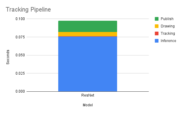
In order to run our tracker faster, we need to understand what the bottleneck is in our tracking pipeline. For this demo, our pipeline has four main steps:

Inference: Running the image through the detection model
Tracking: Running the detections through the tracking algorithm
Drawing: Drawing the tracking bounding boxes on the image
Publishing: Publishing the image back into the image stream The Drawing and Publishing steps are just for viewing the demo, so we will ignore them.


Tracking Pipeline

From the chart below, we can see that the pipeline time is dominated by the model’s inference, with tracking being a very small proportion of the overall. Therefore, if we want to improve our tracking speed we need to run a faster model.


ResNet Tracking Pipeline

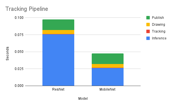
The initial detection model used had a ResNet backbone, which is an accurate but slower model. We can replace it with a mobilenet backbone, which is a model designed for mobile phones, so it is much faster, at the cost of some accuracy. From the chart below, we can see that this change alone almost doubles our speed. We have gone from processing at 10 fps (1 / 0.1) to around 20 fps (1 / 0.05) for tracking.


Model Comparison

To get an intuitive understanding of how big a difference in speed this is, I am displaying the last five detections for each model. We can see how much closer together and tighter around the person the detections at 20 FPS are. For tracking, this means our tracker has less distance between detections, and has less uncertainty regarding prediction.


10 FPS Detections


20 FPS Detections

Now when we run our tracker at 20 FPS, without changing any other parameters, we get a noticeable improvement in performance.


20 FPS Tracking Sequence 1


20 FPS Tracking Sequence 2

There are still some obvious issues with the tracker (e.g. phantom tracks), but we have managed to improve the smoothness overall. However, there are some downsides to using a faster inference model that we need to discuss.

In general, the faster the model, the lower the accuracy. We can see this pattern in the sequences below. The mobilnet model misses a lot more detections than the resnet model. This is particularly noticeable when the pedestrians are further away, as the mobilenet model doesn’t pick them up at all. We need to consider these factors when designing our tracker.


MobileNet Detections


ResNet Detections

Evaluating Tradeoffs

Overall, we are trying to balance speed and accuracy. Faster speed gives us a smoother tracker, and less uncertainty about our predictions, whereas higher accuracy gives us more certainty about our detections. We can think about this as having more recent information or having more accurate information.

There is certainly a minimum level of accuracy required for a tracker to function effectively, but additional accuracy isn’t as valuable due to the persistent nature of the tracked objects. If a detection is missed in one frame, it can be recovered in the next. However, faster tracking is always valuable.

For real time tracking, a simple, fast tracker usually wins over a slower more sophisticated method. For a more detailed discussion, see SORT.

Limitations

The limitations of applying this demo to self-driving cars directly are as follows:

We have used a single class tracker, with only a single class in our images (pedestrians). In order to incorporate this into a self-driving car, we would need to make our tracker multi-class, which would make it slightly more complex.
Our detections and tracks are only in 2D (image bounding boxes). In order to incorporate these tracks into a planning system, we would need to convert them to 3-dimensions. Tracking in 3D is not that much more complicated than 2D, as we just add z-values to our bounding boxes. However, getting fast, and accurate 3D detections is much more challenging.
The ‘fast’ detection model we have used is actually pretty slow, as it is a two-stage detector. If we were to change to a single stage detector designed for speed such as YOLO, or SSD, we might be able to use a more complex tracker and still maintain our 20 FPS benchmark.
In the example scenes, we used a stationary camera. In the real world, the car would be moving which would change how the pedestrians and camera are moving relative to one another. Depending on how fast the car is moving, this can complicate our tracking significantly.


Moving Camera Tracking

Tracking is only one of the first steps for the whole self-driving pipeline. From these tracks we need to predict what the pedestrians and other cars are going to do, and then plan our path through them.
We ignored most of the appearance based metrics for tracking. Incorporating more appearance based methods would help with re-identifying objects returning from occlusion.


Optical Flow Example 2

We didn’t use any deep learning in our tracking. If we use deep learning everything automatically gets better. This is only 50% a joke, DeepSORT.
We skipped over tuning any of the other parameters of the tracker, in favour of discussing the speed. There are many hyperparameters that we can adjust in order to improve not only the tracker, but the detections as well.

Conclusion

Tracking is a useful technique for determining the behaviour of other agents on the road. For self driving applications, a robust, real time tracking pipeline is required. We’ve seen that for real time problems, faster, simpler tracking can work better than slower more complex methods. Tracking is a building block for a prediction system, in order to understand what pedestrians and vehicles will do next.

Reference

Detection

Tracking

Repositories